Chapter 3
Internal forces
3.1 Internal force variables
In the previous chapter, we considered internal forces appearing on the hypothetical cuts. Here we continue discussing internal force variables but with a focus on describing them as a continuous function of the position along the body. From the previous example (Fig. ??), we know how to find the internal forces in the middle of the beam (Eq. ??). However, we can also perform the same procedure for any other section of the beam. Therefore, it makes sense to consider the reaction forces and moments as functions of the coordinate along the beam length (Fig. 3.1).
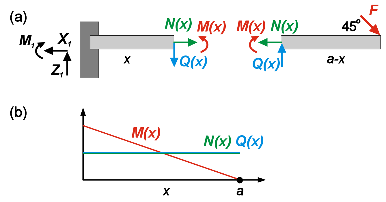
Let us consider a cut located at the distance \(x\) from the left hinge/wall (Fig. 3.1). By balancing forces and moments acting on the left and right fragments, it is easy to show that
\begin {equation} \begin {aligned} N(x)&=F/\sqrt {2} \\ Q(x)&=F/\sqrt {2} \\ M(x)&=\frac {F(a-x)}{\sqrt {2}} \end {aligned} \label {eq:continuousbeam} \end {equation}
Therefore, both longitudinal and shear forces are constant functions of the coordinate \(x\), while moment linearly decreases with an increase in \(x\).
3.2 Distributed loads
Prior to this moment, we have considered only idealized point forces. Now we will consider loads distributed along the region of the body (line loads). We will learn how to search for internal forces without exact knowledge of the reaction forces and move towards governing equation of continuum mechanics in the next Chapter.
Note: In our next derivations, we will heavily rely on a very useful mathematical concept of Taylor expansion of the function. If we have arbitrary function \(f(x)\), then we can try to approximate it in the vicinity of point \(x_0\) using a polynomial function. So we can find the approximate value of \(f(x+\Delta x)\) just knowing the properties of the function in the point \(x_0\). We will skip the strict mathematical discussion of the necessary conditions and restrictions on function \(f\) and value of \(\Delta x\), and just claim that for a small enough \(\Delta x\) and well-behaved function \(f\), the Taylor expansion provides a good approximation of \(f\). For example, the second order approximation of \(f(x+\Delta x)\) can be expressed as \begin {equation} f(x_0+\Delta x)=f(x_0)+\Delta x f'(x_0)+ \frac {1}{2}\Delta x^2 f''(x_0)+O(\Delta x^3) \end {equation} In shorter form the general Taylor expansion can be written as \begin {equation} f(x_0+\Delta x)=\sum _{i=0}^{\infty }\frac {1}{n!}f^{(i)}(x_0)\Delta x^i \end {equation} Note, that \(f^{(i)}\) means \(i-\)th derivative of the function, while \(\Delta x^i\) is a regular power.
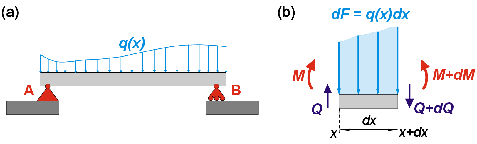
Let us consider a straight beam subjected to line load that can be expressed as a function of the coordinate \(q(x)\) (Fig. 3.2). We select a very small (infinitesimal) beam element of length \(dx\) stretching from coordinate \(x\) to \(x+dx\). Note that here we use \(dx\) instead of \(\Delta x\) to emphasize the infinitesimal length of this piece. Due to that \(dx<<(dx)^2\), and we can use the first order Taylor expansion to find the change in total applied force between left and right ends of the selected beam as \(dF=q(x)dx\). Let us now write equilibrium equation for the small piece, taking into account that we can express the shear force and moment on the right side as \(Q(x+dx)=Q+dQ\) and \(M(x+dx)=M+dM\) respectively. \begin {equation} Q(x)+dQ=Q(x)-q(x)dx \end {equation} We also can write Taylor expansion of \(Q(x)\) at \(x\) as \begin {equation} Q(x)+dQ=Q(x)+\frac {dQ}{dx}dx+... \end {equation} By comparing coefficients in these two equations, we conclude that \begin {equation} q(x)=-\frac {dQ}{dx} \end {equation} This equation establishes the relation between line load and internal shear force in the body. To balance moments, we write \begin {equation} M(x)+dM=M(x)+Q(x)dx \end {equation} Similar to force, we can obtain the first order Taylor expansion and get \begin {equation} q(x)=-\frac {d^2M}{dx^2} \end {equation}
Therefore, we can express \(Q(x)\) and \(M(x)\) via integration as \begin {equation} \begin {aligned} Q(x)&=-\int {q(x)dx}+C_1 \\ M(x)&=\int {Q(x)dx}+C_2 \end {aligned} \label {eq:integrationmoment} \end {equation} Integration constants \(C_1\) and \(C_2\) have to be found from boundary conditions at bearings and intermediate conditions at connections between body parts. Boundary conditions depend on the bearing type. For example, simple hinge implies \(M=0\), and free end provides two boundary conditions \(M=0\) and \(Q=0\) simultaneously. Note that by computing shear force and moment via integration (Eq. ??), we do not need to calculate bearing reactions at all. If we recall Fig. ?? describing the different types of hinges, we can notice that each degree of freedom corresponds to additional equality boundary conditions that can be used to find integration constants (Eq. ??).