Chapter 2
Bearings
2.1 Bearings and degrees of freedom
The condition of static equilibrium that we discussed earlier does not mean that the body is immovable. The body still can translate and rotate; in a two-dimensional case an object can have three kinematics degrees of freedom (DoFs): two orthogonal translational displacements along x- and y- axes, and one rotation around z-axis. The motion of the body can be restricted by eliminating some DoFs with the help of bearings (Fig. 2.1). Depending on the type of bearing, one, two, or all three DoFs can be removed. The kinematic constraints imposed by bearings trigger so-called bearing reactions, or simply reactions. Note that if exactly all degrees of freedom are removed, the system is called statically determinate or isostatic.
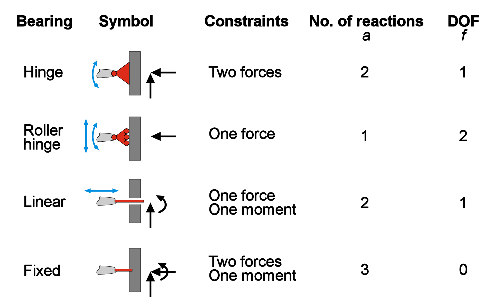
As you can see, the sum of the number of reactions \(a\) and DoFs \(f\) is always equal to 3 (for 2D case). This is a necessary (but not a sufficient!) condition for a statically determinate system with one body. Namely, \begin {equation} \sum _{i}{a}-3=0 \end {equation} For more general 2D system with \(n\) connected bodies \begin {equation} \sum _{i}^{n}{a_i}+\sum {z}-3n=0, \end {equation} where \(z\) is a number of intermediate reaction between movable bodies.
By knowing a number of bodies \(n\), a number of bearing reactions \(a\) and intermediate reactions \(z\), we can distinguish three different cases for 2D force systems defined by the value of \(D\), where \begin {equation} D=\sum _{i}^{n}{a_i}+\sum {z}-3n \label {eq:D} \end {equation} We know that a determinate (or isostatic) system must have \(D=0\) (Fig. 2.2b). If \(D<0\), then the system is movable since it has unrestricted DoF (Fig. 2.2a). If \(D>0\), then the system is called indeterminate or hyperstatic - the system is immovable and contains extra reactions that can be removed (Fig. 2.2c).
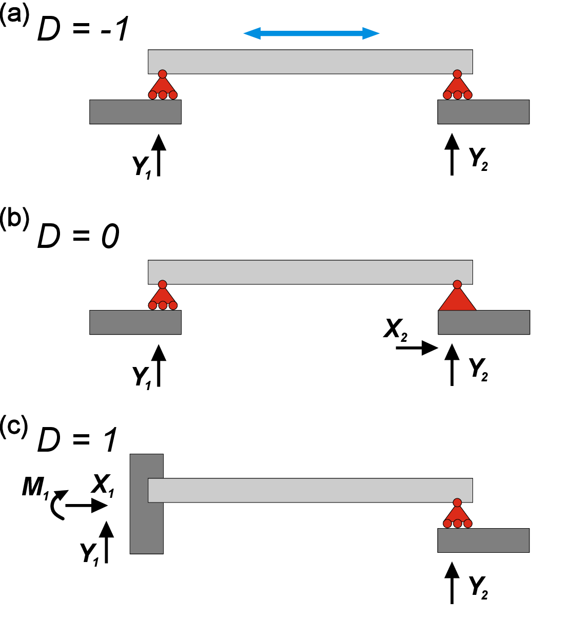
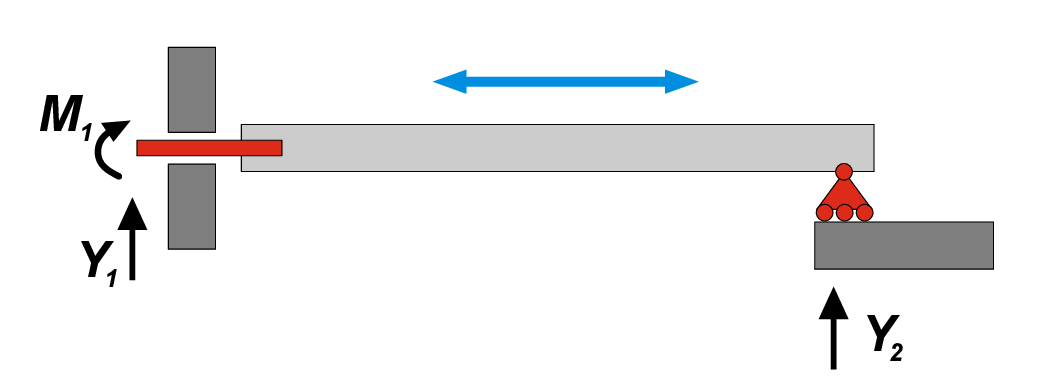
Again, we need to emphasize that above-mentioned mathematical precondition is a necessary, but not sufficient, requirement. One exception from this rule is the system with two and one reactions in the left and right bearings respectively shown in Fig. 2.3. Here, we have \(D=0\), which usually corresponds to determinate system. However, it is clear that the beam can move freely in a horizontal direction, therefore it has 1 DoF! In this specific case, force vectors \(Y_1\) and \(Y_2\) are parallel, and they both can compensate only vertical direction of action, while the horizontal movement is not restricted.
2.2 Free body diagrams
Free body diagrams provide a way to compute forces acting inside the body (internal force variables). By definition, an internal force variable is the resultant of all internal forces in a solid body at a hypothetical cut through the body (Fig. 2.4). If we imagine cutting the body in equilibrium along some line, we technically create two fragments that are no longer in equilibrium. Therefore we need to introduce additional forces on the cut to restore the equilibrium and balance the forces. For a 2D system we can distinguish three resultants on the cut: longitudinal force \(L\) (perpendicular to cut), transverse/shear force \(Q\) (in plane of cut) and bending moment \(M\) (perpendicular to the 2D area of force system). Together with reactions, internal force variables can be determined using a free body diagram.
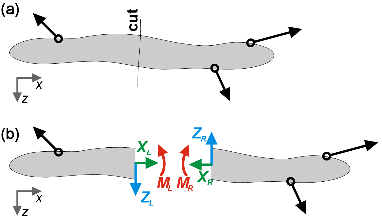
By hypothetically splitting the beam into two fragments, we add six internal force variables on the cut (three for left and three for right) that balance both fragments. To keep the whole body in equilibrium after ”gluing” these two fragments back, the internal force variables on the left and right should have the same amplitude and opposite directions. Therefore, by cutting the beam, we increase the number of bodies to \(n=2\), however, we also add three intermediate reactions \(z\), therefore keeping \(D\) constant (Eq. ??)
Note: To correctly operate with internal force variables, we need to agree on non-ambiguous sign conventions. We will obey the following rules
- An intersection area is called positive if normal vector is in the direction of coordinate vector, and negative otherwise;
- Internal force variable (force or moment) is positive if it is located at a positive intersection area AND if it is in direction with a coordinate vector;
- The moment is regarded as a vector according to the right-hand rule;
- Note that the reactional internal force variable at the corresponding negative intersection is also considered as positive.
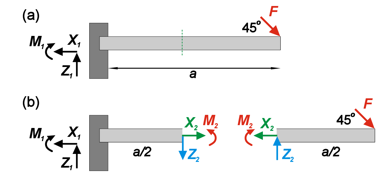
For illustration, we consider an example of a beam with length \(a\), that is fixed on the left end and subjected to an inclined point load \(F\) on the right end (Fig. 2.5). We search for the bearing reactions as well as internal forces in the middle point of the beam. Simply balancing forces and moments we get \begin {equation} \begin {aligned} X_1&=F/\sqrt {2} \\ Y_1&=F/\sqrt {2} \\ M_1&=-Fa/\sqrt {2} \end {aligned} \end {equation} To find the internal forces and moments at the middle of the beam, we need to cut the beam into two fragments, introduce two reaction forces \(X_2\) and \(Z_2\) and one reaction moment \(M_2\) to preserve equilibrium. Finally, by balancing the forces for both fragments we get
\begin {equation} \begin {aligned} X_2&=F/\sqrt {2} \\ Y_2&=F/\sqrt {2} \\ M_2&=\frac {Fa}{2\sqrt {2}} \end {aligned} \label {eq:middlebeam} \end {equation}